MEASUREMENTS
2.1 METHODS
2.1.1 Biomechanical Assessment Procedure
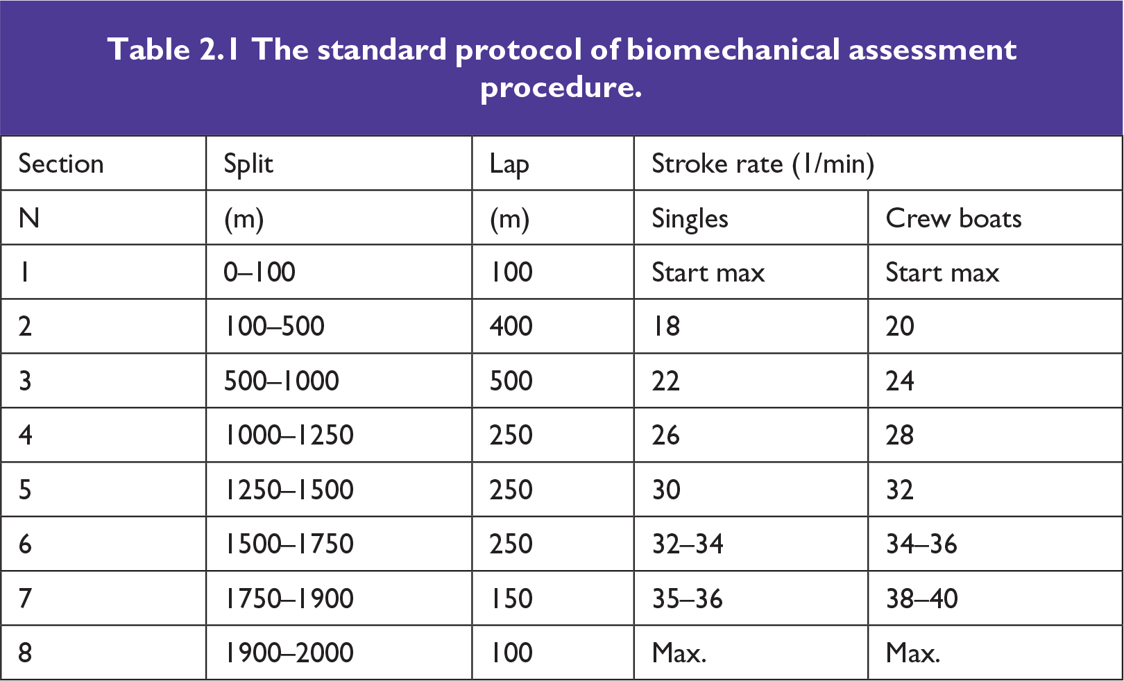
An important part of the biomechanics assessment procedure is the testing protocol, which must provide standard conditions and make results comparable between rowers and over the course of time. There are two major factors affecting rowing technique: the stroke frequency and fatigue. Therefore a test protocol was used consisting of two parts:
■ A step-test with increasing stroke rate: for example, 5–6 sections by 250m or 1 minute at 20, 24, 28, 32, 36 str/min with a free recovery of about 3–5 minutes and 30 second maximal effort;
■ Race length of 2,000m with full effort or specified percentage of it (say, at 95 per cent).
This test protocol was quite time-consuming (1–2 hours) and put a significant load on rowers. Therefore, a combined test protocol was designed, which enabled determination of both effects at once. The test consists of one continuous 2000m piece at racing force application, but various rates (see Table 2.1).
This testing protocol received very positive feedback from rowers and coaches. This test was a good training load itself; the first half of it is performed at aerobic training intensity, which allows smooth transition to the second half with anaerobic intensity; only the last 500m is performed with stroke rates close to those used in racing. There can be some variation of this protocol for junior rowers and veterans. For example, sections N5 and N7 could be replaced with light paddling with corresponding reduction of the stroke rate for the next sections. The data samples are taken and averaged at every lap.
2.1.2 Data Processing
When rowing is measured with any telemetry system, the raw data looks like a long chain of waves where each peak represents one stroke cycle (see Fig. 2.1a). The number of strokes done (usually 200–250 for 2km test) multiplied by the number of channels (for example 48 channels, usually measured in an eight) makes the amount of data overwhelming and difficult to comprehend.
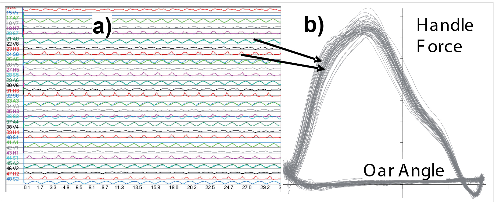
Fig. 2.1 Examples of raw data (a) and averaged force curves at various stroke rates (b).
A common way to represent cyclic rowing data is plotting it as an X–Y chart, where the X coordinate is the oar angle or handle position on a rowing machine. As an example, Fig. 2.1b shows the handle force curve in this way. Though this representation is more understandable and gives some impression about rowing technique, it is not useful for precise numerical evaluation, comparison and modelling of rowing biomechanics.
The key part of the BioRow data analysis is an algorithm of data averaging, which allows the conversion of information collected from an unlimited number of cycles into one typical stroke cycle. It was developed from 1991–199328 and was used for more than 25 years for data analysis both in a boat and on a rowing machine, as well as in other cyclic sports (canoeing and swimming). This method allows effective data analysis, storage and comparison, and very clear feedback and interpretation for rowers and coaches. Here it is explained in essence.
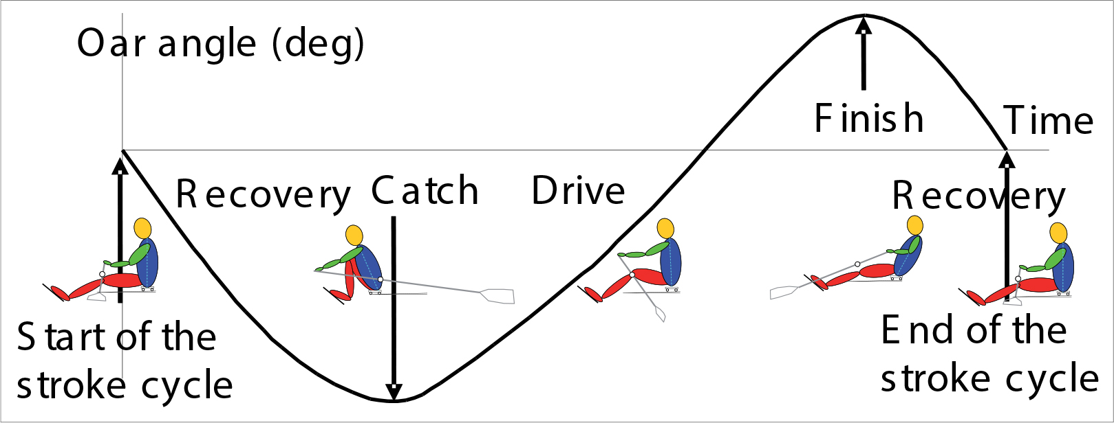
Fig. 2.2 Detection of the stroke cycle.
Firstly, the stroke cycle should be detected (Fig. 2.2). For this, we use oar angle data (or handle position on a rowing machine) and define the start of the stroke cycle at the moment when the angle crosses zero during the recovery (oars perpendicular to the boat axis, or the handle of a rowing machine passing over the knees). This point was chosen as it is the most idle period of the cycle, without sharp changes of the rower’s movement, where it is possible to pause naturally. Some other systems use the catch as the cycle start, which breaks apart this quick and very important phase of the stroke, and makes it difficult to analyse. In addition, it is not natural to pause the stroke at the catch. In crew boats, the cycle is detected using only one oar’s data for the whole crew (usually, of the stroke rower, port side in sculling), which allows perfect synchronisation of the data.
The process of the data averaging starts with detecting the number of stroke cycles in a selected section of rowing, calculating the average stroke rate SRav and its standard deviation SRsd. Then the strokes are filtered, and only the cycles within the range SRav ± k*SRsd are used for averaging (k = 1 is strong filtering, 2 – medium and 3 – light filtering). The filtering is necessary because the high variation of the stroke rate makes typical patterns unreliable: it doesn’t make sense to average rowing at 20 str/m and at 40 str/m.
Cycles of various stroke rates have different numbers of data points: for example, at a 25Hz sampling frequency, the cycle at 20 str/m would have 75 data points, but at 44 str/m only 34 points, which makes such data difficult to handle. Therefore, arrays with a fixed number of points n are used for averaged data (n = 50 was chosen). After filtering, these arrays are created for each data channel and time stamps Ti are assigned to each point, where Ti = (60/SRav)/n. For the raw data, the time from the beginning of the stroke cycle to each data point is different for various strokes (the cycle periods are still slightly different), which means it may belong to different phases of the cycle and should not be averaged. Therefore, raw data is interpolated to derive a value at the time Ti of each point of the averaged array, and then these values are averaged for all cycles in the sample. In other words, durations of raw cycles shrink or stretch on X-axis to fit them to the duration of the average stroke cycle (Fig. 2.3). Also, standard deviations could be derived for each point Ti, which allows evaluation of variability of rowing technique (see Chapter 3.3.3).
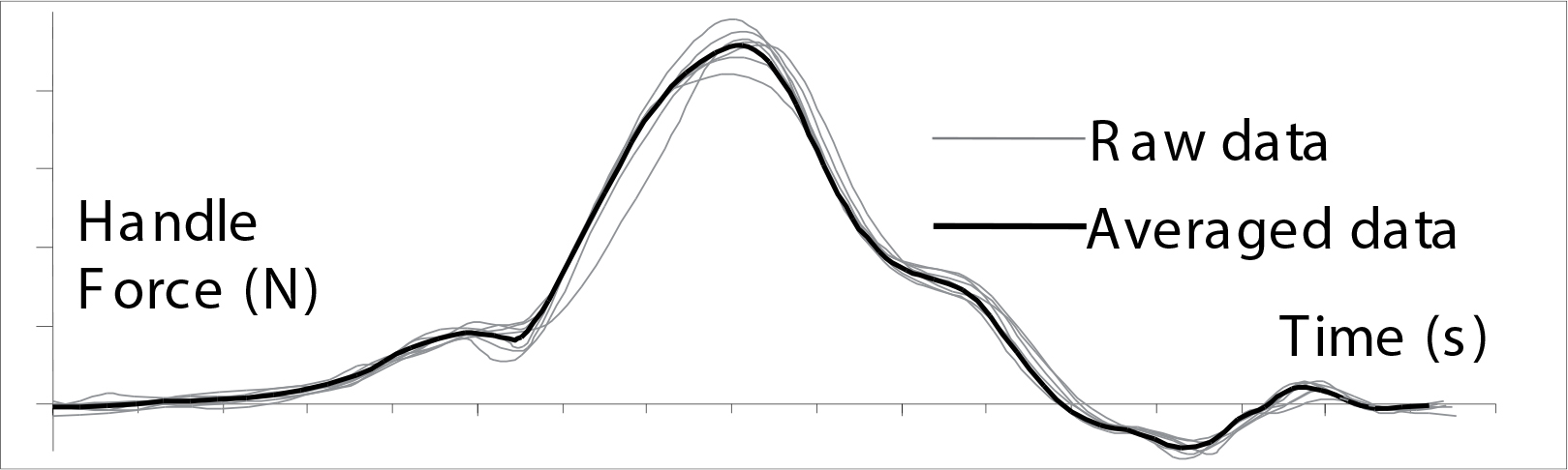
Fig. 2.3 Raw and averaged data of the handle force.
To check the validity of this method, various rowing criteria were derived for every stroke of the raw data (Vraw), then their averaged values (Vraw.av) were compared with the same criteria derived from the averaged arrays Vav. It was found that Vav values were slightly lower than Vraw.av, and for most criteria, the difference was within a range of 0.5 per cent. It is important that for average force the difference was much smaller (0.19 per cent) than for maximal force (1.11 per cent), which could be explained by deviation of the timing of the peaks in each stroke, which makes the average curve smoother with lower peak, but insignificantly affects the area under the curve.
In conclusion, the averaging algorithm works correctly and reliably and provides effective data analysis and feedback in rowing and other cyclic sports.
2.2 TIMING
Time is an absolute universal variable, which has only one dimension and direction. Therefore, timing can be related unambiguously to mechanical variables and make the analysis clear and effective. In rowing and also in many other sports, the result itself is measured in the time taken to cover the race distance.
2.2.1 Stroke Rate and Rowing Speed
Stroke rate (or cadence, frequency, pace, etc.) is the most obvious and commonly used timing variable in rowing as in many other cyclic sports. It is always measured by coaches and rowers during training and races and is used to define training and racing intensity. The stroke rate R is defined as a number of strokes N per unit of time T:
| R = N / T | (1) |
where T is in minutes – the commonly accepted unit of time in rowing, and R is strokes per minute denoted as 1/min, or min−1. Together with stroke length and force, the stroke rate is one of three components of rowing power, so it is one of the main determinants of performance in rowing. However, it is not possible to increase the stroke rate to infinity to improve rowing results; it is limited by mechanical conditions (inertial losses of energy increase with the stroke rate) and with neuromuscular abilities of rowers (a higher stroke rate would require a faster muscle contraction, which may be inefficient, and quicker coordination of movements). Therefore, it is important to find the optimal stroke rate, which maximizes rowing speed. This optimum may be different for different crews and boat types. Fig. 2.4 shows an example for two crews: in Crew A the maximal rowing speed was achieved at a stroke rate of 32 min−1, while in Crew B it continues to grow up to and beyond 40 min− 1.
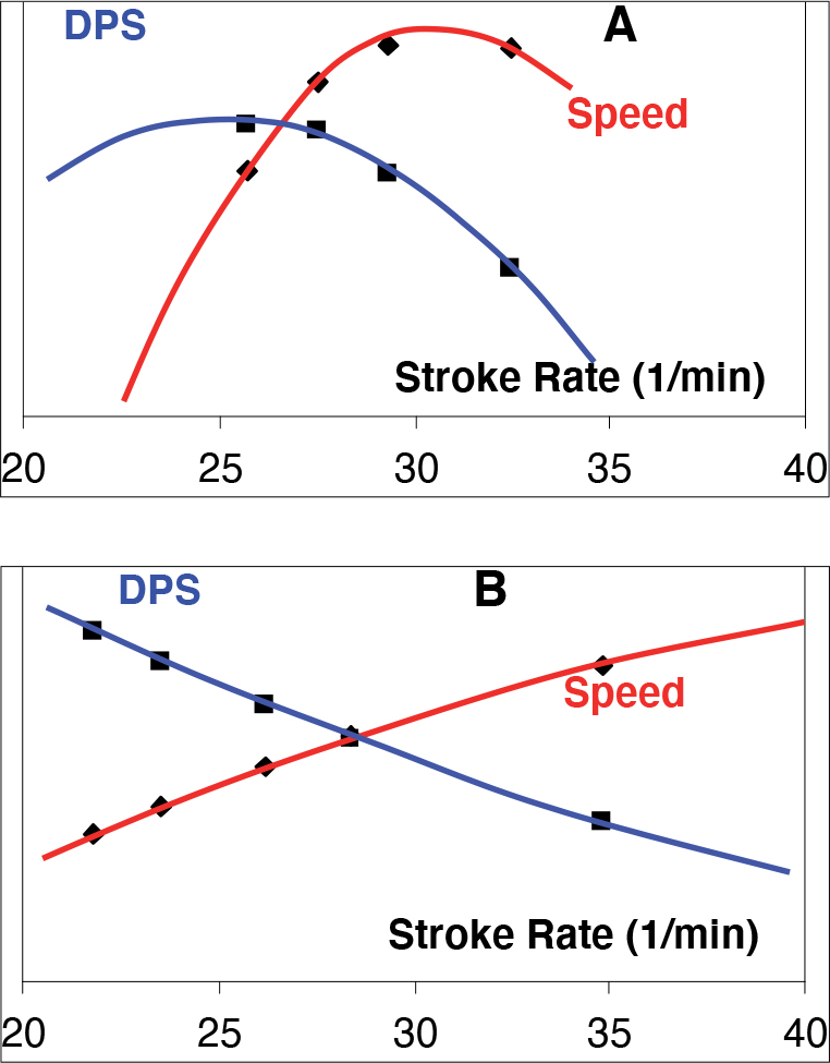
Fig. 2.4 The effect of the stroke rate on the rowing speed and distance per stroke (DPS) in two rowing crews.
To evaluate dependence of the rowing speed on stroke rate and find its optimum, we introduced a method36 based on effective work per stroke (EWPS). Previously, distance per stroke DPS was used as a measure of the stroke effectiveness. However, DPS always decreases at higher stroke rates (even in the best crews), because the duration of the stroke cycle becomes shorter.
So, the question was: ‘What do we need to preserve as the stroke rate increases?’ It was decided that the main objective is to sustain the application of force F, of stroke length L, and of mechanical efficiency E. The effective work per stroke, EWPS, integrates all these variables and is used as the basis of the method:
| EWPS ∼ F * L * E | (2) |
The rowing speed V and rowing power P are related as following:
| P = DF * V3 | (3) |
where DF is some dimensionless factor depending on the boat type, displacement, weather conditions and blade efficiency. Therefore, EWPS can be expressed in terms of power P, stroke cycle time T, rowing speed V, stroke rate R:
| EWPS = P T = P (60 / R) = 60 DF (V3/ R) | (4) |
For the two sections of rowing with different stroke rates (R1 and R2), if the value of EWPS was maintained constant and also DF1 and DF2 are the same, then ratio of the rowing speeds (V1 and V2) must be:
| V1 / V2 = (R1 / R2)1/3 | (5) |
This means the rowing speed is proportional to the cube root of the stroke rate: if the stroke rate is doubled at constant EWPS, the boat speed increases only by about 26 per cent (21/3 = 1.26), and to double the boat speed, the stroke rate must be eight times higher.
Correspondingly, the ratio of DPS (distance per stroke) values can be expressed as:
| DPS1 / DPS2 = (R2 / R1)2/3 | (6) |
This means the distance per stroke is inversely proportional to the square of the cube root of the stroke rate: if the stroke rate is doubled, DPS shortens by about 37 per cent (0.52/3 = 0.63).
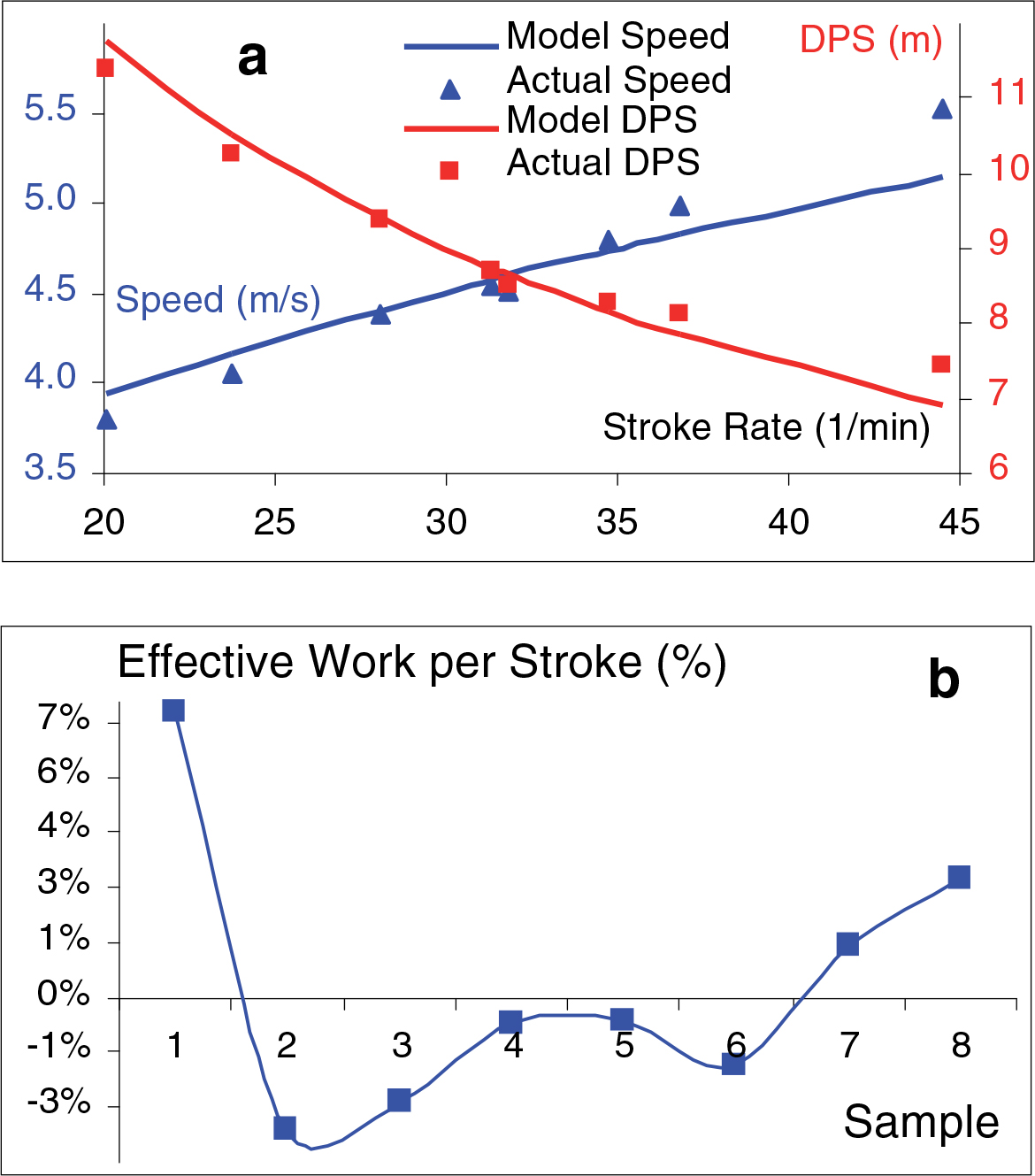
Fig. 2.5 Dependence of the rowing speed and DPS on the stroke rate (a), analysis of EWPS (b).
To use this method, we do not need to know drag factor DF, because it is assumed constant for all samples analysed. However, this is applicable only for the same boat, rowers and weather conditions, which is a limitation of the method. Fig. 2.5a illustrates the equations and represents dependencies of the rowing speed and DPS on the stroke rate.
The most practically convenient application of the method is the definition of ‘prognostic’ or ‘model’ value of the speed Vm for every stroke rate:
| Vm = V0 (R1 / R0) 1/3 | (7) |
where V0 is usually average of all samples of the race or step-test. Then, the actual speed in each sample Vi can be compared with the ‘model’ Vm and its deviation D calculated:
| D = Vi / Vm − 1 | (8) |
If D is positive, then EWPS in this sample was relatively higher than average over the whole race or test (Fig. 2.5b) and vice versa. This method can be used for race analysis in cyclic water sports (rowing, swimming,20 canoeing), employed for evaluation of the strength- and speed-endurance using a step-test and does not require sophisticated equipment (only a stopwatch or StrokeCoach).
On an ergometer, as the drag factor for speed calculation is always constant (in Concept2 erg DF = 2.8). This method is applicable without any limitations and can be used for developing normative splits for ergo training. To do this, the target speed V0 and stroke rate R0 should be defined firstly, then
| D = Vi / Vm − 1 | (9) |
should be used to calculate normative splits for various stroke rates. For example, your target for a 2km ergo race is 6:00 at the rate of 36 min − 1. If you can train at the rate 18 at a split of 1:53, this means your muscles are ready to produce the same amount of work per stroke, as required for your target result and rate.
2.2.2 Rowing Rhythm
The standard definition of rhythm is the ratio of the drive time to the total time of the stroke cycle (50 per cent means a 1/1 ratio of the drive to recovery times). It was found that the rhythm has a strong positive correlation (r = 0.89) with the stroke rate (Fig. 2.4) because possibilities to shorten the drive are limited. This happens because rowers increase the stroke rate mainly by means of shortening recovery time, which is much easier to do than decrease the drive time. However, the stroke rate only explains 79 per cent of the rhythm variation (Fig. 2.6) and 21 per cent depends on other factors.
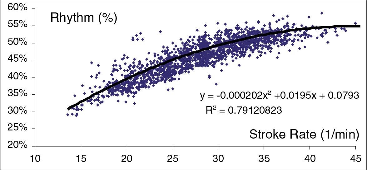
Fig. 2.6 Dependence of the rowing rhythm on the stroke rate.
The standard deviation of residuals from the trend (n = 2881) was σ = 2.5 per cent, which means that at the same stroke rate the rhythm may vary within ± 7.5 per cent (± 3σ) in various crews. For example at a stroke rate of 32.5 str/min the average rhythm based on the above trend is 50 per cent, but it could be between 42.5 per cent and 57.5 per cent.
2.2.3 Case Study: Factors Affecting the Rhythm
Is it better to have the rowing rhythm higher or lower? Many coaches believe that a lower rhythm is more efficient and ask their crews to shorten the drive time, but does that make sense? Biomechanical variables of two M1x were analysed at the same stroke rate of 32.5 str/min (Fig. 2.7). Sculler 1 (red) had a rhythm of 49.5 per cent or 0.91s drive time compared to Sculler 2’s (blue) 52.5 per cent and 0.97s correspondingly; that is, the second one had a 3 per cent higher rhythm and 0.06s longer drive time. The reason for this difference was quite simple: Sculler 1 had a total oar angle of 107.5 degrees while Sculler 2 had 116 degrees; that is he had an 8.5 degree longer stroke length. This fully explains the difference in rhythm and drive time since the average handle velocity during the drive (= drive length / time) had the same value of 1.73 m/s in both scullers. This happened in spite of Sculler 1 applying a 3.9 per cent higher maximal force and 2.6 per cent higher average force than Sculler 2.
What other biomechanical features are related to this difference in rhythm and stroke length? During the recovery, Sculler 2 has to move the handle much faster (Fig. 2.7, point 1) to cover a longer distance in a shorter time, so his average handle speed was 11.7 per cent higher. This was impossible without faster seat/leg movement (2). At the catch, Sculler 2 changes direction of the seat movement much quicker than Sculler 1, slightly before his handles change direction (3). Contrarily, Sculler 1 uses his trunk even before the catch (4). Consequently, the boat acceleration of Sculler 2 has an earlier and deeper negative peak (5), but higher first positive peak (6), so his boat and stretcher move relatively faster (7), creating a better platform for acceleration of Sculler 2’s mass (‘trampoline effect’, see Chapter 3.2.5).
Other technical advantages of Sculler 2 were:
■ More effective return of the trunk at the finish (8);
■ Better blade work at the catch (9) and finish (10);
■ Faster force increase up to 70 per cent of max. (11);
■ 1.5 per cent lower variation of the boat velocity (0.5s gain over 2km);
■ 3.3 per cent higher rowing power because of longer drive.
As a result, the rowing speed of Sculler 2 was 5.9 per cent higher (6:34 for 2km) than Sculler 1 (6:57) as well as his performance (world medallist compared to third finalist for Sculler 1). Conclusion:The rhythm and drive time cannot be changed voluntarily as they depend on the stroke rate, length and rowing speed. The stroke length is the main factor affecting the rhythm. There are other factors, which may affect rhythm (shape of the force curve and depth of the blade), which we may study in the future.
2.3 ANGLES
2.3.1 Horizontal Oar Angle and Drive Length
The horizontal oar angle is one of the most important variables in rowing biomechanics, which defines the amplitude of the oar movement in a horizontal plane. It is measured from the perpendicular position of the oar relative to the boat axis, which is zero degrees (Fig. 2.8a). The catch angle is defined as the minimal negative angle, the finish angle is the maximal positive angle and the total angle is the difference between finish and catch angles. The horizontal oar angle is used for triggering the stroke cycle, which occurs at the moment of zero oar angle during recovery.
The oar angle can be measured at the oar shaft or at the gate, and these two methods produce slightly different results (Fig. 2.8b). The total angle measured at the gate was found to be 4–5 degrees larger than the total oar angle, mainly because of finish angles. There are two main reasons for this difference (Fig. 2.9):
Fig. 2.8 Definitions of the horizontal oar angles (a), comparison of the angle measurements at the oar and at the gate (b).
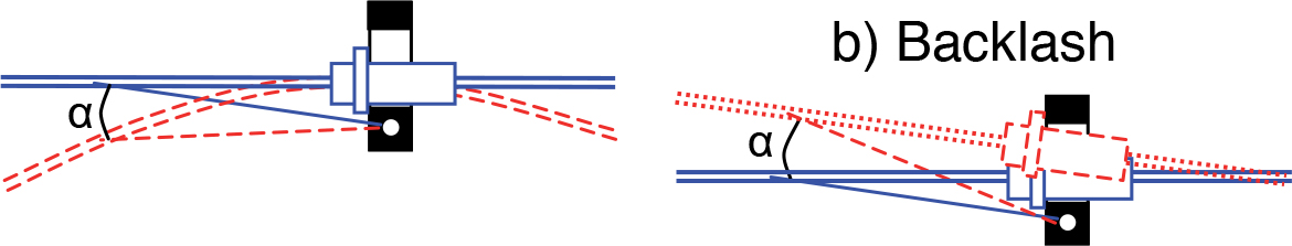
Fig. 2.9 Differences in measurements of the oar angle at the oar shaft and at the gate.
1. A bend of the oar shaft. When force increases at the first half of the drive, the oar shaft bends and its angular velocity is slightly faster than at the gate. At the second half of the drive the oar extends, and its rotation appears to be slower than the gate rotation. This is the reason for the small difference in the catch angle and has no effect on the finish angle, because the force at this point is minor.
2. Backlash of the oar sleeve in the gate is the main contributor to the difference in the finish angle. It depends on the geometry of the gate, sleeve and button, and also on coordination of feathering along with horizontal and vertical movements of the oar. The backlash does not create any inefficiency because the blade is already out of the water and no propulsive force is produced at that moment.
The method of measuring the angle (at the oar, or at the gate) usually corresponds to the method of measuring the force and is determined by the following factors:
■ If the target is the geometry and kinetics of the rower’s movement then the oar angle and force are the best choice. The main advantage of this method is accurate determination of the handle position and power production of the rower.
■ If boat kinetics and propulsive forces need to be measured then gate angle and force are quite useful for defining force components at the pin. However, the rower’s power cannot be estimated accurately because of unknown actual leverage of the oar.
The drive length is defined as the length of the arc Larc made by the middle of the handle, and related to the amplitude of horizontal angle A and actual inboard Lin.a as:
| Larc = A Lin.a π / 180 | (10) |
The actual inboard Lin.a is the distance from the pin (centre of the oar rotation) to the middle of the handle, and it is related to the normally measured inboard Lin (from the collar to the top of the handle) as:
| Lin.a = Lin + Wg/2 − Wh/2 | (11) |
where Wg/2 is half the gate width (2cm for the standard gate) and Wh/2 is half the handle width, which is set at a standard 6cm in sculling and 15cm in rowing. It is important to maintain this standard, because it makes drive length comparable in sculling and rowing, and is used for calibration of the handle force and provides correct calculations of work per stroke and rowing power.
| F = m a | (12) |
| P = m * ω = fhnd * Lin-a * ω | (13) |
| Fhnd = fgate* (Lout-a / (Lin-a + Lout-a)) | (14) |
| Fgate = fpin * cos α | (15) |
| Fprop = Fpin - Fstr | (16) |
| FPF − FSH = mb ab − FD | (17) |
| FSH − FH = mR aR | (18) |
| FD (V) = DF*Vb2 | (19) |
| Fsus = Fg − (Fs + FSV) | (20) |
| Fc = mt vt2/ r | (21) |
| Fg.n = Fh.n + Fb.n = Fh.n Lout.a / (Lout.a + Lin.a) | (22) |
| G = lout / lin | (23) |
| P = DF v3 | (24) |
| P = W / t = F L / t = F v | (24) |
| Ppin = t ω = (t / rin) (ω Rin) = fh Vh | (25) |
| Pprop = fprop VCM | (26) |
| Prower = Phandle + Pfoot = Fhandle Vhandle + Ffoot Vfoot | (27) |
| R1 / R2 = F2 / F1 = Fs / Fh = Fg / Fh = k | (28) |
| k = (Rin 1 Rout) / Rout ∼ 1.44 | (29) |
| Pt ∼ Vt (0.59 Fh + 0.41 Fs) | (30) |
| WpS 5D ∫ F ΔL = ∫ M Δϕ | (31) |
| P = WpS / t = WpS R/60 | (32) |
| J = FT = m v | (33) |
| Ek = 0.5 m v2 = W = p T ≈ F L (simplified) | (34) |
| P = a HR2 + b HR + c | (35) |
End of sample. Continue to next page to purchase book.

